• Resources for learning RNN.
• Backpropagation Through Time in detail.

LSTMs and GRUs, variants of vanilla RNNs, have proven extremely effective in Computer Vision and Natural Language Processing applications. Of all the excellent resources on RNNs available online, following are the ones that helped me understand them clearly:

1. Understanding LSTM Networks: Clear explanation with block diagrams.

2. Recurrent Neural Networks Tutorial, Part 1 to Part 3: Tutorial in Theano with a touch of BPTT and vanishing/exploding gradient problem.

3. The Unreasonable Effectiveness of Recurrent Neural Networks: Types of sequence problems and fun applications in NLP.

4. Awesome Recurrent Neural Networks: A curated list of RNN resources.

Backpropagation Through Time

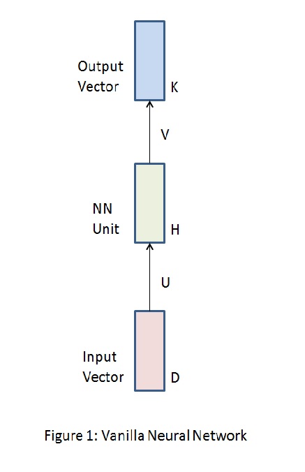
$Figure\;1$ shows a vanilla neural network architecture. $D$ dimensional input vector is connected to the neural network unit through weights $U$. The neural network unit is in turn connected to the $K$ dimensional output vector through weights $V$. The neural network unit consists of a single layer of $H$ neurons with $tanh$ activation. Gradients for optimization of this network can be computed using standard back propagation.

RNNs, on the other hand, allow mapping between variable length input sequences to variable length output sequences. Thus, gradients need to be back propagated in time to update weights. Depending on the type of application, RNN sequences can be broadly categorized (Refer Andrej Karpathy’s blog) into:

1. Synchronised input and output sequences

2. Unsynchronised input and output sequences

3. Input sequences

4. Output sequences

Synchronized input and output sequences

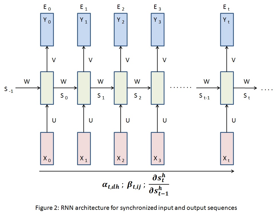
Extending vanilla neural network architecture from $Figure\;1$, $Figure\;2$ shows a sequence of neural network units mapping the input sequences $X_{i}$s to output sequences $Y_{i}$s. Such architecture finds place in frame level video classification where the prediction depends on the current frame as well as the frames that appeared before it. $S_{i}$s are the $H$ dimensional output of the hidden layer in the neural network units. These are the memory of the network which transfer previous state information along the chain. The neural network unit at $t+1$ takes input from $X_{t}$ throught $U$ and $S_{t}$ through $W$. Weights $U$, $V$ and $W$ are shared across RNN units. $S_{-1}$ is initialized to a vector of zeros.

The total loss for the above RNN is:

$$E = \sum_{t=0}^T E_t \tag{1}\label{1}$$

where $T$ is the length of input and output sequences. $\frac{\partial E}{\partial v_{hk}}$, $\frac{\partial E}{\partial u_{dh}}$, $\frac{\partial E}{\partial w_{ij}}$ are the target gradients that need to be computed.

For RNN unit at $t$, compute the following:

$$\frac{\partial E_{t}}{\partial y^k_{t}} \tag{2}\label{2}$$ $$\frac{\partial E_{t}}{\partial s^h_{t}} = \sum_{k=1}^K \frac{\partial E_{t}}{\partial y^k_{t}}\frac{\partial y^k_{t}}{\partial s^h_{t}} \tag{3}\label{3}$$ $$\alpha_{t,dh} = \frac{\partial s^h_{t}}{\partial u_{dh}} + \frac{\partial s^h_{t}}{\partial s^h_{t-1}}\alpha_{t-1,dh} \tag{4}\label{4}$$ $$\beta_{t,ij} = \frac{\partial s^j_{t}}{\partial w_{ij}} + \frac{\partial s^j_{t}}{\partial s^j_{t-1}}\beta_{t-1,ij} \tag{5}\label{5}$$

Finally,

$$\frac{\partial E_{t}}{\partial v_{hk}} = \frac{\partial E_{t}}{\partial y^k_{t}}\frac{\partial y^k_{t}}{\partial v_{hk}} \tag{6}\label{6}$$ $$\frac{\partial E_{t}}{\partial u_{dh}} = \frac{\partial E_{t}}{\partial s^h_{t}}\alpha_{t,dh} \tag{7}\label{7}$$ $$\frac{\partial E_{t}}{\partial w_{ij}} = \frac{\partial E_{t}}{\partial s^j_{t}}\beta_{t,ij} \tag{8}\label{8}$$

where,

$$k \in \{1,2,3....K\}; \;i,j,h \in \{1,2,3....H\}; \;d \in \{1,2,3....D\}$$ $$\alpha_{-1,dh} = 0; \;\beta_{-1,ij} = 0; \;s^h_{-1} = 0$$

$\alpha_{t,dh}, \;\beta_{t,ij}$ and $\frac{\partial s^h_{t}}{\partial s^h_{t-1}}$ are messages passed along the RNN as shown in $Figure\;2$.

Unsynchronized input and output sequences

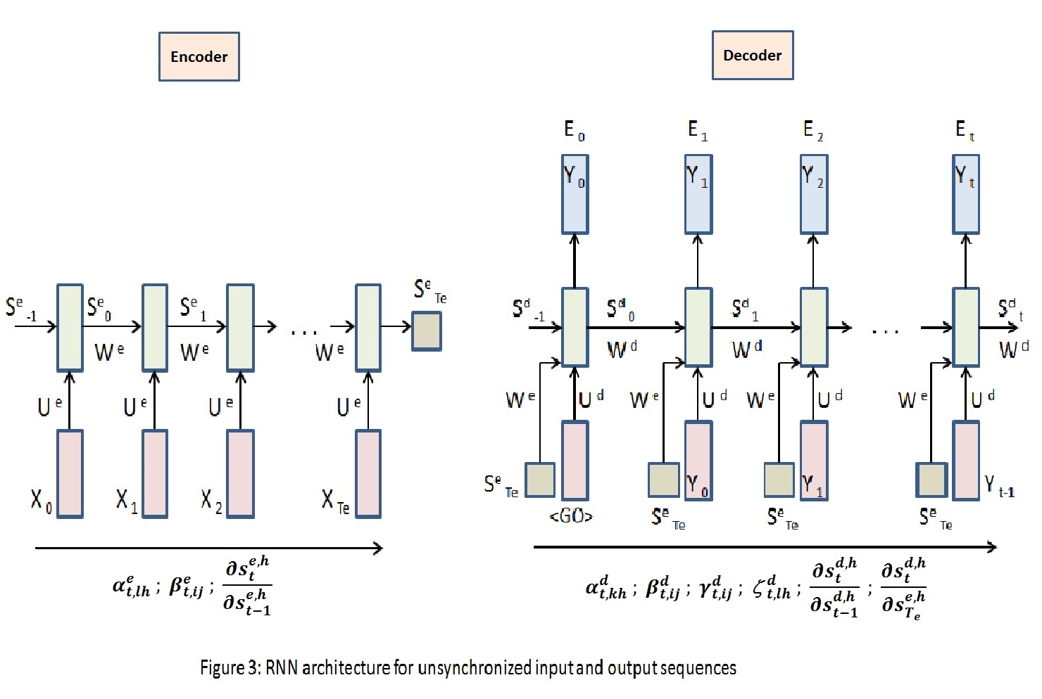
RNNs are pretty successful in machine translation applications. The architecture in $Figure\;3$ shows an encoder RNN connected to a decoder RNN through the encoder’s hidden state $S^e_{Te}$, where $Te$ is length of the input sequence to the encoder. The RNN decoder unit at $t+1$ takes $S^e_{Te}$, $Y_{t}$ and $S^d_{t}$ as inputs. In this architecture, a variable length input sequence can be mapped to a variable length output sequence. Generally, encoders and decoders use different sets of parameters as shown. Each neural network unit in the encoder and the decoder consist of a single hidden layer of $H$ neurons.

The total loss is given by equation $(\ref{1})$ and the target gradients that need to be computed are $\frac{\partial E}{\partial v^d_{hk}}$, $\frac{\partial E}{\partial u^d_{kh}}$, $\frac{\partial E}{\partial w^d_{ij}}$, $\frac{\partial E}{\partial u^e_{lh}}$ and $\frac{\partial E}{\partial w^e_{ij}}$, where superscripts $e$ and $d$ represent parameters for encoders and decoders respectively.

For encoder compute:

$$\alpha^e_{t,lh} = \frac{\partial s^{e,h}_{t}}{\partial u^e_{lh}} + \frac{\partial s^{e,h}_{t}}{\partial s^{e,h}_{t-1}}\alpha^e_{t-1,lh} \tag{9}\label{9}$$ $$\beta^e_{t,ij} = \frac{\partial s^{e,j}_{t}}{\partial w^e_{ij}} + \frac{\partial s^{e,j}_{t}}{\partial s^{e,j}_{t-1}}\beta^e_{t-1,ij} \tag{10}\label{10}$$

For decoder compute:

$$\frac{\partial E_{t}}{\partial y^k_{t}} \tag{11}\label{11}$$ $$\frac{\partial E_{t}}{\partial s^{d,h}_{t}} = \sum_{k=1}^K \frac{\partial E_{t}}{\partial y^k_{t}}\frac{\partial y^k_{t}}{\partial s^{d,h}_{t}} \tag{12}\label{12}$$ $$\alpha^d_{t,kh} = \frac{\partial s^{d,h}_{t}}{\partial u^d_{kh}} + \frac{\partial s^{d,h}_{t}}{\partial s^{d,h}_{t-1}}\alpha^d_{t-1,kh} \tag{13}\label{13}$$ $$\beta^d_{t,ij} = \frac{\partial s^{d,j}_{t}}{\partial w^d_{ij}} + \frac{\partial s^{d,j}_{t}}{\partial s^{d,j}_{t-1}}\beta^d_{t-1,ij} \tag{14}\label{14}$$ $$\zeta^d_{t,lh} = \frac{\partial s^{d,h}_{t}}{\partial s^{e,h}_{T_e}}\alpha^e_{T_e,lh} + \frac{\partial s^{d,h}_{t}}{\partial s^{d,h}_{t-1}} \zeta^d_{t-1,lh} \tag{15}\label{15}$$ $$\gamma^d_{t,ij} = \frac{\partial s^{d,j}_{t}}{\partial w^e_{ij}} + \frac{\partial s^{d,j}_{t}}{\partial s^{e,j}_{T_e}}\beta^e_{T_e,ij} + \frac{\partial s^{d,j}_{t}}{\partial s^{d,j}_{t-1}}\gamma^d_{t-1,ij} \tag{16}\label{16}$$

Hence,

$$\frac{\partial E_{t}}{\partial v^d_{hk}} = \frac{\partial E_{t}}{\partial y^k_{t}}\frac{\partial y^k_{t}}{\partial v^d_{hk}} \tag{17}\label{17}$$ $$\frac{\partial E_{t}}{\partial u^d_{kh}} = \frac{\partial E_{t}}{\partial s^{d,h}_{t}}\alpha^d_{t,kh} \tag{18}\label{18}$$ $$\frac{\partial E_{t}}{\partial w^d_{ij}} = \frac{\partial E_{t}}{\partial s^{d,j}_{t}}\beta^d_{t,ij} \tag{19}\label{19}$$ $$\frac{\partial E_{t}}{\partial u^e_{lh}} = \frac{\partial E_{t}}{\partial s^{d,h}_{t}}\zeta^d_{t,lh} \tag{20}\label{20}$$ $$\frac{\partial E_{t}}{\partial w^e_{ij}} = \frac{\partial E_{t}}{\partial s^{d,j}_{t}}\gamma^d_{t,ij} \tag{21}\label{21}$$

where,

$$k \in \{1,2,3....K\}; \;i,j,h \in \{1,2,3....H\}; \;l \in \{1,2,3....D\}$$ $$\alpha^e_{-1,lh} = 0; \;\beta^e_{-1,ij} = 0; \;s^{e,h}_{-1} = 0$$ $$\alpha^d_{-1,kh} = 0; \;\beta^d_{-1,ij} = 0; \;\gamma^d_{-1,ij} = 0, \;\zeta^d_{-1,lh} = 0; \;s^{d,h}_{-1} = 0$$

$\alpha^e_{t,lh}$ and $\beta^e_{t,ij}$ are messages passed across the encoder. These are then accumulated and passed across the decoder through $\zeta^d_{t,lh}$ and $\gamma^d_{t,ij}$. Information in the form of $\alpha^d_{t,kh}$ and $\beta^d_{t,ij}$ also flow through the decoder for gradient computation.

Input sequences

In sentiment analysis, a sequence of words is classified into positive or negative sentiments. $Figure\;4$ shows the architecture for such applications.

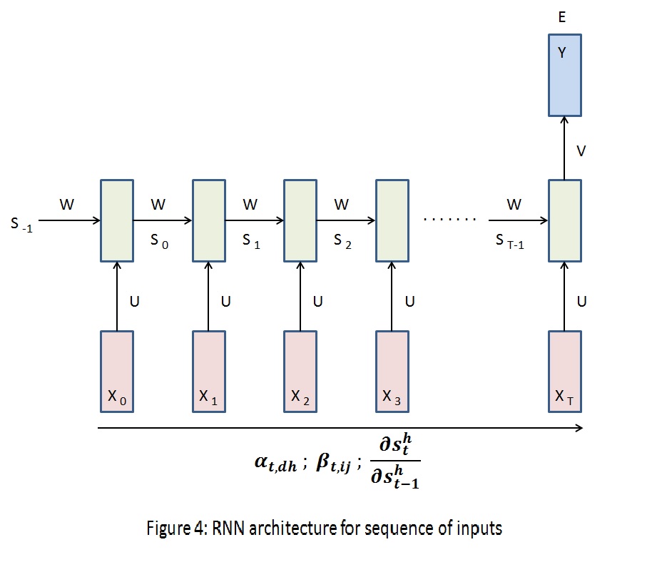
Gradient computations are very straight forward in this case.

$$\frac{\partial E}{\partial y^k} \tag{22}\label{22}$$ $$\frac{\partial E}{\partial s^h_{T}} = \sum_{k=1}^K \frac{\partial E}{\partial y^k}\frac{\partial y^k}{\partial s^h_{T}} \tag{23}\label{23}$$

And,

$$\frac{\partial E}{\partial v_{hk}} = \frac{\partial E}{\partial y^k}\frac{\partial y^k}{\partial v_{hk}} \tag{24}\label{24}$$ $$\frac{\partial E}{\partial u_{dh}} = \frac{\partial E}{\partial s^h_{T}}\alpha_{T,dh} \tag{25}\label{25}$$ $$\frac{\partial E}{\partial w_{ij}} = \frac{\partial E}{\partial s^j_{T}}\beta_{T,ij} \tag{26}\label{26}$$

where $\alpha_{t,dh}$ and $\beta_{t,ij}$ are given by equations $(\ref{4})$ and $(\ref{5})$ respectively.

$$k \in \{1,2,3....K\}; \;i,j,h \in \{1,2,3....H\}; \;d \in \{1,2,3....D\}$$ $$\alpha_{-1,dh} = 0; \;\beta_{-1,ij} = 0; \;s^h_{-1} = 0$$

Output sequences

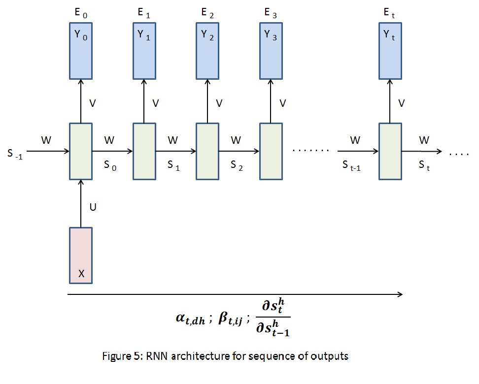
Image captioning takes an image and outputs a sequence of words, RNN architecture for the same is shown in $Figure\;5$. Refer equations $(\ref{2})$, $(\ref{3})$, $(\ref{5})$ for $\frac{\partial E_{t}}{\partial y^k_{t}}$, $\frac{\partial E_{t}}{\partial s^h_{t}}$ and $\beta_{t,ij}$ respectively. Target gradients $\frac{\partial E}{\partial v_{hk}}$, $\frac{\partial E}{\partial u_{dh}}$, $\frac{\partial E}{\partial w_{ij}}$ can be computed using $(\ref{6})$, $(\ref{7})$ and $(\ref{8})$. $\alpha_{t,dh}$, however, is computed as below:

$$\alpha_{t,dh} = \frac{\partial s^h_{t}}{\partial s^h_{t-1}}\alpha_{t-1,dh} \tag{27}\label{27}$$

where,

$$\alpha_{0,dh} = \frac{\partial s^h_{0}}{\partial u_{dh}} \tag{28}\label{28}$$ $$k \in \{1,2,3....K\}; \;i,j,h \in \{1,2,3....H\}; \;d \in \{1,2,3....D\}$$ $$\alpha_{-1,dh} = 0; \;\beta_{-1,ij} = 0; \;s^h_{-1} = 0$$

Conclusion

We have seen how the chain rule of calculus can be used to compute gradients in RNNs for various applications. The process can be viewed as passing messages through RNNs across time. Optimize weights using HF optimization to avoid ‘vanishing gradinets’ problem. Gradient computations for LSTMs, GRUs and other RNN variants require a similar approach.